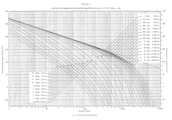
DESCRIPCIÓN

This model is described in Recommendation 369-9 of the ITU-R. This is a empirical propagation method used to medium wave broadcasting radio-planning.

This model should be used for the determination of ground-wave field at frequencies between 10 kHz and 30 MHz.

This model is based on a group of measurements carried out for different frequencies, ground types, and climates.

DESARROLLO

The measurements are shown in a ground-wave propagation curves group, and they are calculated under specified assumptions:

They refer to smooth homogenous spherical Earth

In the troposphere, the refractive index decrease exponentially with height, as describes in Recommendation 453 of the ITU-R.

Both the transmitting and receiving antennas are at ground level.

The radiating element is a short vertical monopole. Assuming such a vertical antenna to be on the surface of a perfectly conducting plane Earth, and excited so as to radiate 1 kW, the field strength at a distance of 1km would be 300 mV/m.

The curves are drawn for distances measured around the curved surface of the Earth.

The curves give the value of the vertical field-strength component of the radiation field, ie. that which can be effectively measured in the far-field region of the antenna.

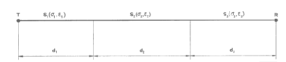
If the signal is propagated along a path without changes in the terrain features (homogeneous path) these curves are directly applied using the interpolations needed (depending on the frequency and distance from the receiving point to the transmitting antenna).

In the case of a situation of mixed propagation paths (heterogeneous smooth earth), the Milington method is used to determine the field strength.

The mixed paths can consist on the sections S1, S2, S3 with lengths of d1, d2, d3, etc., Whose conductivity and permittivity are σ1, ε1; σ2, ε2; σ3, ε3, as shown in the illustration for three sections:

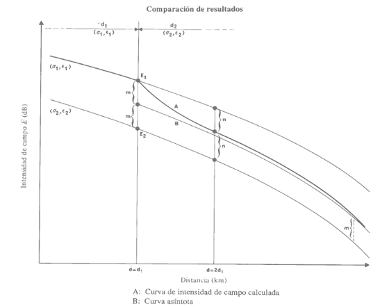
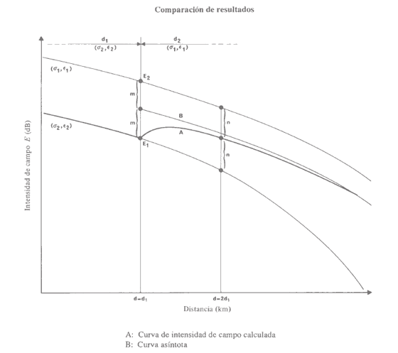
To apply the Millington method curves or the different types of terrain of sections S1, S2, S3, etc. are considered available, Then, for a particular frequency, the curve for section S1 is chosen, and determining the value of field strength E1(d1) in dB (mV / m) to the distance d1. With the curve for section S2 the field strength E2(d1) y E2(d1 + d2) is determined and, proceeding in the same way with the curve corresponding to the S3 section, the field strength E3(d1 + d2) y E3(d1 + d2 + d3) is defined and so on.

Equation (1) defines a field strength received ER:

ER = E1(d1) - E2 (d1) + E2 (d1 + d2 ) - E3(d1 + d2 ) + E3(d1 + d2 + d3)

Is inverted after the procedure, called R to the transmitter and T to the receiver, reaching a ET field intensity defined by the equation:

ET = E3 (d3 ) - E2 (d3) + E2 (d3 + d2 ) - E1(d3 + d2 ) + E1(d3 + d2 + d1)

The field strength required is ½ [ER + ET], and it was evident how to extend the computation to a larger number of sections.

To compute with precision is necessary to have a conductivity map of the terrain that define him, this map the conductivity is introduced into the calculation by a Morphographic layer, in the case of not having conductivity map can enter a conductivity default parameters calculation, considering the path like an homogeneous path.

Parameterization of the calculation method

In Sirenet a mechanism to include the possible additional losses due to uneven terrain on signal propagation has been implemented. Thus, besides transmitted power, frequency and terrain conductivity, the possible obstacles between transmitter and reception point will affect to received field level. This mechanism is based on studies conducted by universities and research institutions that propose to estimate potential losses depending on the uneven terrain and propose a procedure for calculation. Specifically, Sirenet is based on study [2].

While these procedures are not standardized or recognized at technical level on the international stage, they can be applicable in practical cases in which, experimentally, technicians have demonstrated by field measurements the influence of significant obstacles on signal propagation.

This mechanism for calculating potential losses introduced by obstacles is presented as a complement to the method of surface curves propagation discussed in Recommendation 368-9 of the ITU-R [1]. Losses are modeled with adjustable parameters (depending on the height of the obstacle in wavelengths) so that the user can adjust the results to a particular environment conditions.

APLICATIONS

•This model is not accurate for zones where there are a large number of deterministic obstacles.

•It is commonly used in Half Wave service for long-distance predictions.

•It is very fast, because it interpolates values previously stored.

REFERENCES

[1] Recommendation ITU-R P.368-9, "Ground-wave propagation curves for frequencies between 10 kHz and 30 MHz".

[2] "Estimation of the single obstacle attenuation in MF band from field data". Susana López, David de la Vega, David Guerra, Gorka Prieto, Manuel Velez, and Pablo Angueira.

Department of Electronics & Telecommunications. Bilbao Engineering College (University of the Basque Country). Alameda Urquijo s/n. 48013 Bilbao. SPAIN.