DESCRIPTION

The ITU-R Recommendation P.1411 [1] provides guidance on outdoor short-range propagation over the frequency range 300 MHz to 100 GHz. Information is given on path loss models for line-of-sight (LoS) and non-line-of-sight (NLoS) environments. The propagation methods are applicable for distances up to 1 km, affected primarily by buildings and trees, rather than by variations in ground elevation. The effect of buildings is predominant, since most short-path radio links are found in urban and suburban areas. The propagation models of these methods are symmetric in the sense that they treat radio terminals at both ends of a path in the same manner. From the model’s perspective, it does not matter which terminal is the transmitter and which is the receiver.

DEVELOPMENT

Physical operating environments and definition of cell types

The Recommendation identifies five environments: Urban very high-rise, urban high-rise, urban low-rise/suburban, residential and rural. For each of the five different environments two possible scenarios for the mobile are considered. Therefore the users are subdivided into pedestrian and vehicular users. For these two applications the velocity of the mobile is quite different yielding different Doppler shifts.

The type of propagation mechanism that dominates depends also on the height of the base station antenna relative to the surrounding buildings. Table 1 lists the typical cell types relevant for outdoor short-path propagation.

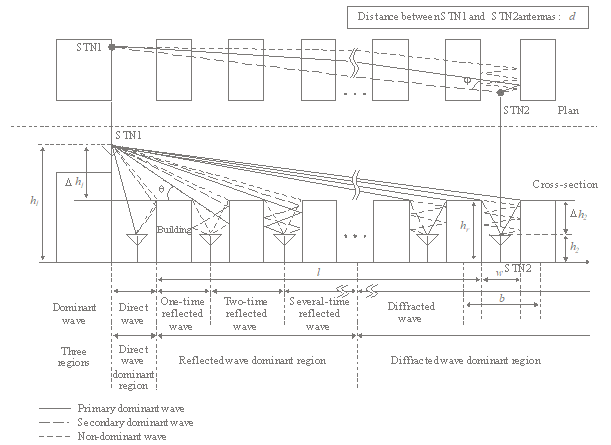
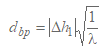
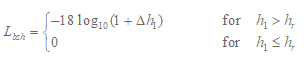
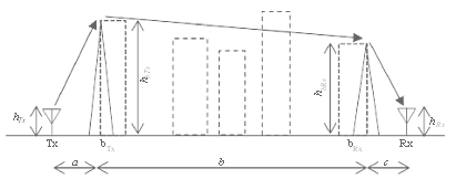
Table 1: Definition of cell types

Path categories

Three levels of the location of the station can be considered. They are 1) over the roof-top; 2) below roof-top but above head level; and 3) at or below head level. Comprehensively, six different kinds of links can be considered depending on the locations of the stations, each of which may be LoS or NLoS. The parameters relevant for an NLoS over the roof-top path are defined in the following and represented in Figure 1.

Figure 1: Definition of parameters for the NLoS over-the-roof case

The relevant parameters for this situation are:

hr:        average height of buildings (m)
w:        street width (m)
b:        average building separation (m)
φ:        street orientation with respect to the direct path (degrees)
h1:        Station 1 antenna height (m)
h2:        Station 2 antenna height (m)
λ:        length of the path covered by buildings (m)
d:        distance from Station 1 to Station 2.

Figure 2 depicts the situation for a typical dense urban micro-cellular NLoS-case In this case the base station antennas are below the roof-top level.

Figure 2: Definition of parameters for the NLoS below the roof-top case

The relevant parameters for this situation are:

w1:        street width at the position of the Station 1 (m)
w2:        street width at the position of the Station 2 (m)
x1:        distance Station 1 to street crossing (m)
x2:        distance Station 2 to street crossing (m)
α:        is the corner angle (rad).

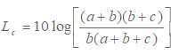
Models for propagation within street canyons (below the roof-top situations)

This site-general model is applicable to situations where both the transmitting and receiving stations are located below-rooftop, regardless of their antenna heights. The site-general model is provided by the following equation:

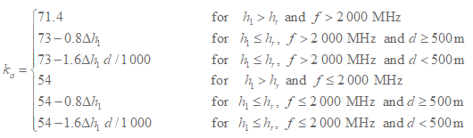
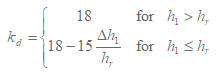
where:

d :        3D direct distance between the transmitting and receiving stations (m)
f :        operating frequency (GHz)
α :        coefficient associated with the increase of the path loss with distance
β :        coefficient associated with the offset value of the path loss
γ :        coefficient associated with the increase of the path loss with frequency
N(0,σ):        a zero mean Gaussian random variable with a standard deviation σ (dB).

The recommended values for LoS and NLoS situations to be used for below-rooftop propagation in urban and suburban environments are provided in Table 2.

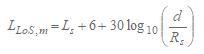
Table 2. Path loss coefficients for below-rooftop propagation

Site-specific model for LoS situation

UHF propagation

In the UHF frequency range, basic transmission loss, can be characterized by two slopes and a single breakpoint.

According to the free-space loss curve, a median value LLoS,m is given by:

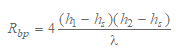
where Rbp is the breakpoint distance in m and is given by:

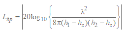
Lbp is a value for the basic transmission loss at the break point, defined as:

SHF propagation up to 15 GHz

At SHF, for path lengths up to about 1 km, road traffic will influence the effective road height and will thus affect the breakpoint distance. This distance, Rbp, is estimated by:

where hs is the effective road height due to such objects as vehicles on the road and pedestrians near the roadway. Hence hs depends on the traffic on the road. The hs values given in Tables 3 and 4 are derived from daytime and night time measurements, corresponding to heavy and light traffic conditions, respectively. Heavy traffic corresponds to 10 20% of the roadway covered with vehicles, and 0.2 1% of the footpath occupied by pedestrians. Light traffic is 0.1 0.5% of the roadway and less than 0.001% of the footpath occupied. The roadway is 27 m wide, including 6 m wide footpaths on either side.

TABLE 3. The effective height of the road, hs (heavy traffic)

TABLE 4. The effective height of the road, hs (light traffic)

When h1, h2 > hs, the approximate values of the upper and lower bounds of basic transmission loss for the SHF frequency band can be calculated using equations (2) and (4), with Lbp given by:

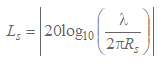
On the other hand, when h1 ≤ hs o h2 ≤ hs no breakpoint exists. When two terminals are close (d < Rs), the basic propagation loss is similar to that of the UHF range. When two terminals are far, the propagation characteristic is such that the attenuation coefficient is cubed.

The basic propagation loss Ls is defined as:

Rs in equation (7) has been experimentally determined to be 20 m.

Based on measurements, a median value is given by:

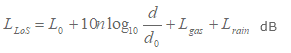
Millimetre-wave propagation

At frequencies above about 10 GHz, the breakpoint distance Rbp in equation is far beyond the expected maximum cell radius (500 m). This means that no fourth-power law is expected in this frequency band. Hence the power distance decay rate will nearly follow the free-space law with a path-loss exponent of about 1.9-2.2.

With directional antennas, the path loss when the boresights of the antennas are aligned is given by:

where n is the path loss exponent, d is the distance between Station 1 and Station 2 and L0 is the path loss at the reference distance d0. For a reference distance d0 at 1 m, and assuming free-space propagation L0=20 log10 f −28 where f is in MHz. Lgas and Lrain, are attenuation by atmospheric gases and by rain which can be calculated from Recommendation ITU-R P.676 and Recommendation ITU R P.530, respectively.

Values of path loss exponent n are listed in Table 5.

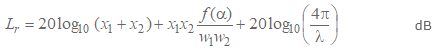
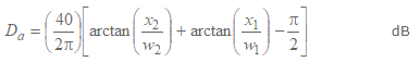
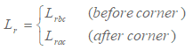
TABLE 5. Directional path loss coefficients for millimetre-wave propagation

Site-specific model for NLoS situations

Frequency range from 800 to 2 000 MHz

For NLoS2 situations where both antennas are below roof-top level, diffracted and reflected waves at the corners of the street crossings have to be considered (see Fig. 2).

where:

Lr :        reflection path loss defined by:

where:

where 0.6 < α [rad] < π.

Ld :        diffraction path loss defined by:

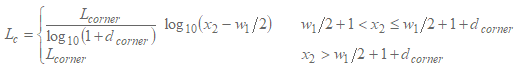
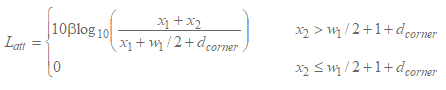
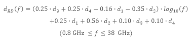
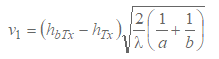
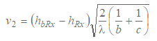
Frequency range from 2 to 38 GHz

Using x1, x2, and w1, as shown in Fig. 2, the overall path loss (LNLoS2) beyond the corner region (x2 > w1/2 + 1) is found using:

where LLoS is the path loss in the LoS street for x1 (> 20 m), as calculated in § 3.1.2. In equation (17), Lcorner is given as 20 dB in an urban environment and 30 dB in a residential environment. And dcorner is 30 m in both environments.

In equation (18), β = 6 in urban and residential environments for wedge-shaped buildings at four corners of the intersection. If a particular building is chamfered at the intersection in urban environments, β is calculated by equation (19).

where f is frequency in MHz.

Models for propagation over roof-tops

This site-general model is applicable to situations where one of the stations is located above-rooftop and the other station is located below-rooftop, regardless of their antenna heights. The site-general model is the same as equation (1) described for the site-general model for propagation below-rooftop (within street canyons).

The recommended values for LoS and NLoS situations to be used for above-rooftop propagation in urban and suburban environments are provided in Table 6.

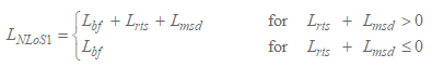
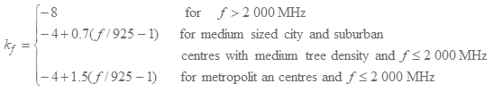
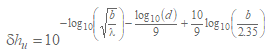
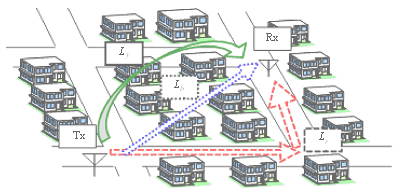
TABLE 6. Path loss coefficients for above-rooftop propagation

Site-specific model

NLoS signals can arrive at the station by diffraction mechanisms or by multipath which may be a combination of diffraction and reflection mechanisms. This section develops models that relate to diffraction mechanisms.

Propagation for urban area

The models are valid for:

h1:        4 to 50 m
h2:        1 to 3 m
f:        800 to 5 000 MHz
 2 to 16 GHz for h1 < hr and w2 < 10 m (or sidewalk)
d:        20 to 5 000 m.

Propagation for suburban area

The model is valid for:

hr:        any height m
Δh1:        1 to 100 m
Δh2:        4 to 10 (less than hr) m
h1:        hr + Δh1 m
h2:        hr − Δh2 m
f:        0.8 to 38 GHz
w:        10 to 25 m
d:        10 to 5 000 m

Millimetre-wave propagation

Millimetre-wave signal coverage is considered only for LoS and NLoS reflection situations because of the large diffraction losses experienced when obstacles cause the propagation path to become NLoS. The frequency range (f) for the suburban area propagation model is applicable up to 38 GHz.

Urban area

The multi-screen diffraction model given below is valid if the roof-tops are all about the same height. Assuming the roof top heights differ only by an amount less than the first Fresnel-zone radius over a path of length l (see Fig. 1), the roof top height to use in the model is the average roof top height. If the roof-top heights vary by much more than the first Fresnel zone radius, a preferred method is to use the highest buildings along the path in a knife-edge diffraction calculation, as described in Recommendation ITU-R P.526, to replace the multi-screen model.

In the model for transmission loss in the NLoS1-case (see Fig. 1) for roof-tops of similar height, the loss between isotropic antennas is expressed as the sum of free-space loss, Lbf, the diffraction loss from roof-top to street Lrts and the reduction due to multiple screen diffraction past rows of buildings, Lmsd.

In this model Lbf and Lrts are independent of the station antenna height, while Lmsd is dependent on whether the station antenna is at, below or above building heights.

The free-space loss is given by:

where:

 d :        path length (m)
 f :        frequency (MHz).

The term Lrts describes the coupling of the wave propagating along the multiple-screen path into the street where the mobile station is located. It takes into account the width of the street and its orientation.

where:

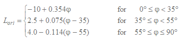
Lori is the street orientation correction factor, which takes into account the effect of roof-top-to-street diffraction into streets that are not perpendicular to the direction of propagation (see Fig.1).

The multiple screen diffraction loss from Station 1 due to propagation past rows of buildings depends on the antenna height relative to the building heights and on the incidence angle. A criterion for grazing incidence is the “settled field distance”, ds:

where (see Fig. 1):

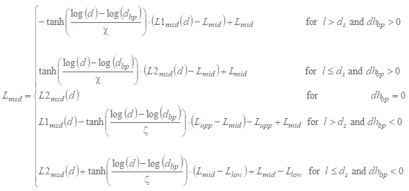
For the calculation of Lmsd, ds is compared to the distance l over which the buildings extend. The calculation for Lmsd uses the following procedure:.

The overall multiple screen diffraction model loss is given by:

where:

and

υ = [0,0417]

χ = [0,1]

where the individual model losses, L1msd(d) and L2msd(d), are defined as follows:

Calculation of L1msd for l > ds

where:

is a loss term that depends on the antenna height:

Calculation of L2msd for l < ds

In this case a further distinction has to be made according to the relative heights of the antenna and the roof-tops:

where:

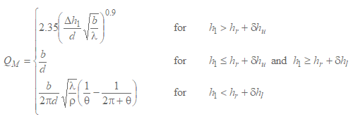
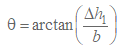
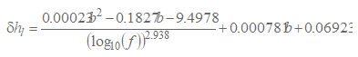
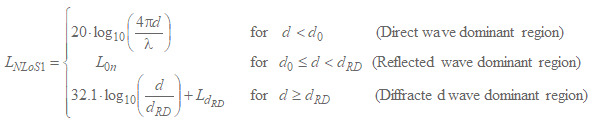
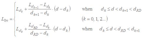
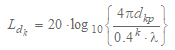
Suburban area

The loss due to the distance between isotropic antennas can be divided into three regions in terms of the dominant arrival waves at Station 2. These are the direct wave, reflected wave, and diffracted wave dominant regions. The loss in each region is expressed as follows based on GO.

where:

Models for propagation between terminals located from below roof-top height to near street level

The models described below are intended for calculating the basic transmission loss between two terminals of low height in urban or residential environments.

The model includes both LoS and NLoS regions, and models the rapid decrease in signal level noted at the corner between the LoS and NLoS regions. The model is valid for frequencies in the 300 3 000 MHz range. The model is based on measurements made with antenna heights between 1.9 and 3.0 m above ground, and transmitter-receiver distances up to 3 000 m.

The parameters required are the frequency f (MHz) and the distance between the terminals d (m).

Step 1: Calculate the median value of the line-of-sight loss:

Step 2: For the required location percentage, p (%), calculate the LoS location correction:

Step 3: Add the LoS location correction to the median value of LoS loss:

Step 4: Calculate the median value of the NLoS loss:

Lurban depends on the urban category and is 0 dB for suburban, 6.8 dB for urban and 2.3 dB for dense urban/high-rise.

Step 5: For the required location percentage, p (%), add the NLoS location correction:

N-1(.) is the inverse normal cumulative distribution function.

Step 6: Add the NLoS location correction to the median value of NLoS loss:

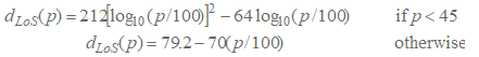
Step 7: For the required location percentage, p (%), calculate the distance dLoS for which the LoS fraction FLoS equals p:

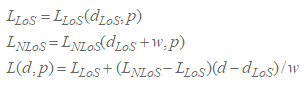
Step 8: The path loss at the distance d is then given as:

a)        If d < dLoS, then L(d, p) = LLoS(d, p)
b)        If d > dLoS + w, then L(d, p) = LNLoS(d, p)
c)        Otherwise linearly interpolate between the values LLoS(dLoS, p) and LNLoS(dLoS + w, p):

The width w is introduced to provide a transition region between the LoS and NLoS regions. This transition region is seen in the data and typically has a width of w = 20 m.

Site-specific model in urban environments

This site-specific model consists of LoS, 1-Turn NLoS, and 2-Turn NLoS situations in rectilinear street grid environments. This model is based on measurement data at frequencies: 430, 750, 905, 1 834, 2 400, 3 705 and 4 860 MHz with antenna heights between 1.5 and 4.0 m above ground. The maximum distance between terminals is up to 1 000 m.

LoS situation

The propagation loss is the same to that in § 3.1.2.

NLoS situations

1-Turn NLoS propagation

A 1-Turn NLoS situation between Station 1 and Station 2 is due to a single corner along the route between Station 1 and Station 2. The distance between the corner and Station 1 is denoted by x1 and the distance between the corner and Station 2 is denoted by x2.

The path loss in this situation can be calculated by:

where LLoS is the path loss with distance d = x1 + x2, as calculated in § 3.1.1, and S1 is a scattering/diffraction parameter calculated by:

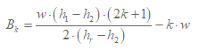
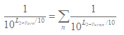
with an operating frequency f in Hz.

2-Turn NLoS propagation

In this case the street path between both stations has two corners. It is possible to establish multiple travel route paths for a 2 Turn NLoS link; thus, the received signal power gain (from Station 1 to Station 2) is calculated considering all 2-Turn route paths. Since received power gain and path loss are logarithmically and inversely related, the received power gain can be written by:

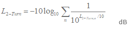
where L2-Turn is the overall pass loss from Station 1 and Station 2, and L2-Turn,n denotes the path loss along with the nth 2-Turn route path. Therefore,

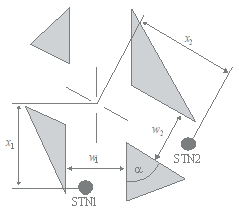
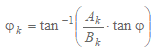
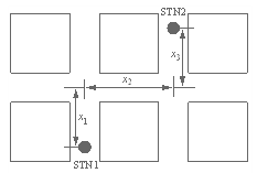
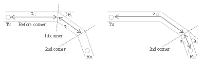
To calculate the path loss along the nth route path, i.e. L2-Turn,n in equation (67), we consider a 2 Turn NLoS situation is depicted in Fig. 3. This link path situation is characterized by three distance components: x1, x2 and x3, where:

x1 denotes the distance between Station 1 and the first corner,
x2 denotes the distance between the first corner and the second corner,
x3 denotes the distance between the second corner and Station 2.

Figure 3: 2-Turn NLoS link between Station 1 and Station 2

Then, the propagation path loss between Station 1 and Station 2 is calculated by:

where LLoS is the path loss with distance d=x1,n+x2,n+x3,n, as calculated in § 3.1.2. S1 is a scattering/diffraction parameter for the first corner turn obtained by (66), and S2 is a parameter for the second corner turn effect calculated by:

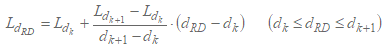
Site-specific model in residential environments

Figure 4 describes a propagation model that predicts whole path loss L between two terminals of low height in residential environments as represented by equation (70) by using path loss along a road Lr, path loss between houses Lb, and over-roof propagation path loss Lv. Lr, Lb, and Lv are respectively calculated by equations (71)-(72), (73), and (74)-(80). Applicable areas are both LoS and NLoS regions that include areas having two or more corners. This model is recommended for frequencies in the 2-26 GHz range. The maximum distance between terminals d is up to 1 000 m. The applicable road angle range is 0-90 degrees. The applicable range of the terminal antenna height is set at from 1.2 m to hBmin, where hBmin is the height of the lowest building in the area (normally 6 m for a detached house in a residential area).

Figure 4: Propagation model for paths between terminals located below roof-top height

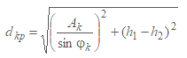
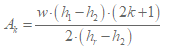
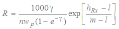
The relevant parameters for this model are:

d:        distance between two terminals (m)
λ:        wavelength (m)
f:        frequency (GHz)
θi:        road angle of i-th corner (degrees)
x1i:        road distance from transmitter to i-th corner (m)
x2i:        road distance from i-th corner to receiver (m)
R:        mean visible distance (m)
hbTx:        height of nearest building from transmitter in receiver direction (m)
hbRx:        height of nearest building from receiver in transmitter direction (m)
hTx:        transmitter antenna height (m)
hRx:        receiver antenna height (m)
a:        distance between transmitter and nearest building from transmitter (m)
b:        distance between nearest buildings from transmitter and receiver (m)
c:        distance between receiver and nearest building from receiver (m).

Figures 5 and 6 below respectively describe the geometries and the parameters. The mean visible distance R is calculated by equations (81)-(84). In the equations, n is the building density (buildings/km2), m is the average building height of the buildings with less than 3 stories (m), l is the lowest building’s height, which is normally 6 (m), and l3 is the height of a 3 story building, which is normally 12 (m).

Figure 5: Road geometry and parameters (example for two corners)

Figure 6: Side view of building geometry and parameters

REFERENCES

[1] ITU-R Rec. P.1411-9, “Propagation data and prediction methods for the planning of short-range outdoor radiocommunication systems and radio local area networks in the frequency range 300 MHz to 100 GHz”, ITU, Geneva, Switzerland, 2017