 |
|
<< Pulse para mostrar la Tabla de Contenidos >> ITU-R REC. P.1812 |


|
|
|
<< Pulse para mostrar la Tabla de Contenidos >> ITU-R REC. P.1812 |
|
|
DESCRIPTION The ITU-R Rec. P.1812 [1] “A path-specific propagation prediction method for point-to-area terrestrial services in VHF and UHF bands” describes a propagation prediction method suitable for terrestrial point-to-area services in the frequency range 30 MHz to 3 GHz for the signal levels detailed evaluation exceeded for a given percentage of time, p%, in the range 1% ≤ p ≤ 50% and a given percentage of locations, pL, in the range 1% ≤ pL ≤ 99%. The method provides detailed analysis based on the terrain profile. Therefore, this method may be used to predict both the service area and availability for a desired signal level (coverage), and the reductions in this service area and availability due to undesired, co- and/or adjacent-channel signals (interference). The method is suitable for predictions for radiocommunication systems utilizing terrestrial circuits having path lengths from 0.25 km up to about 3000 km distance, with both terminals within approximately 3 km height above ground. DEVELOPMENT The method is first described in terms of calculating basic transmission loss (dB) not exceeded for p% time for the median value of locations. The location variability and building entry loss elements are then characterized statistically with respect to receiver locations. The availability of detailed terrain profiles, usually extracted from a digital terrain data base, is assumed. Otherwise, the ITU-R Rec. 1546 should instead be used for predictions. The following input data are required: •Frequency f [GHz]. •Percentage of average year (p) for which the calculated signal level is exceeded. •Percentage of locations (pL) for which the calculated signal level is exceeded. •Geographical coordinates of both terminals (transmitter and receiver) and antenna centre heights above ground level. •Antenna gains Gt, Gr (dBi) in the horizon direction along the great-circle path for both stations. •Type of terrain: Coastal land, inland or sea. •Distances from terminals to the coast. •Radiometeorological data as: oΔN (N-units/km), the average radio-refractive index lapse-rate through the lowest 1 km of the atmosphere. oß0(%), the time percentage for which refractive index lapse-rates exceeding 100 N-units/km can be expected in the first 100 m of the lower atmosphere, used to estimate the relative incidence of fully developed anomalous propagation at the latitude under consideration. It is calculated from the type of terrain and distances to the coast. oN0 (N-units), the sea-level surface refractivity. From this initial set of data, a number of secondary parameters related to effective Earth radius and ducting incidence are calculated, as well as others obtained from the path profile analysis. The propagation prediction method takes into consideration the following elements: •Line of sight. •Diffraction (embracing smooth-Earth, irregular terrain and sub-path cases). •Tropospheric scatter. •Anomalous propagation (ducting and layer reflection/refraction). •Height-gain variation in clutter. •Location variability. •Building entry losses. The different elements are briefly described below. For a detailed calculations description, please refer to the Recommendation [1].
Line-of-sight propagation (including short-term effects) The following should all be evaluated for both line-of-sight and trans-horizon paths. The basic transmission loss due to free-space propagation is given by:
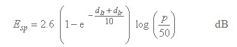
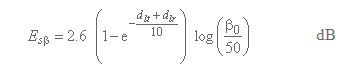
Corrections for multipath and focusing effects at p and ß0 percentage times, respectively, are given by:
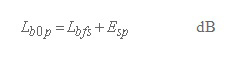
Calculate the basic transmission loss not exceeded for time percentage, p%, due to line-of-sight propagation (regardless of whether or not the path is actually line-of-sight), as given by:
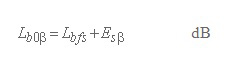
alculate the basic transmission loss not exceeded for time percentage, ß0 %, due to line-of-sight propagation (regardless of whether or not the path is actually line-of-sight), as given by:
Detailed calculations for X, Y, F and G can be found in [1]. Expressions are not reproduced in this document because of their complexity and the wide availability of ITU recommendations.
Propagation by diffraction Diffraction loss is calculated by a method based on the Deygout construction for a maximum of three edges. The principal edge always exists, identified as the profile point having the highest value of diffraction parameter, ν. Secondary edges may also exist on the transmitter and receiver sides of the principal edge. The knife-edge losses for the edges which exist are then combined with an empirical correction. This method provides an estimate of diffraction loss for all types of path, including over-sea or over-inland or coastal land, and irrespective of whether the path is smooth or rough. The above method is always used for median effective Earth radius. In the general case where p < 50%,the calculation must be performed a second time for an effective Earth-radius factor equal to 3. This second calculation gives an estimate of diffraction loss not exceeded for ß0% time. The diffraction loss not exceeded for p% time, for 0.001% ≤ p ≤ 50%, is then calculated using a limiting or interpolation procedure.
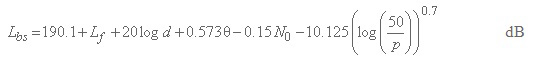
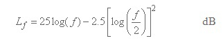
Propagation by tropospheric scatter The basic transmission loss due to troposcatter, Lbs (dB) not exceeded for any time percentage, p, below 50%, is given by:
•Lf : frequency dependent loss.
•N0: path centre sea-level surface refractivity.
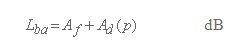
Propagation by ducting/layer reflection The basic transmission loss associated with ducting/layer-reflection not exceeded for p % time, Lba (dB), is given by:
•Af: total of fixed coupling losses (except for local clutter losses) between the antennas and the anomalous propagation structure within the atmosphere. •Ad(p): time percentage and angular-distance dependent losses within the anomalous propagation mechanism.
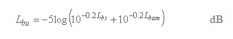
Basic transmission loss not exceeded for p% time and 50% locations ignoring the effects of terminal clutter A detailed procedure should be applied to results of the foregoing calculations for all paths, in order to compute the basic transmission loss not exceeded for p% time and 50% locations. In order to avoid physically unreasonable discontinuities in the predicted notional basic transmission losses, the foregoing propagation models must be blended together to get modified values of basic transmission losses in order to achieve an overall prediction for p% time and 50% locations. After a few intermediate calculations, the basic transmission loss not exceeded for p% time and 50% locations ignoring the effects of terminal clutter, Lbu (dB), is given by:
where: Lbs: basic transmission loss due to troposcatter not exceeded for p% time. Lbam: modified basic transmission loss taking diffraction and line-of-sight ducting/layer-reflection enhancements into account.
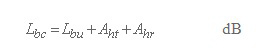
Terminal clutter losses When the transmitter or receiver antenna is located below the height Rt or Rr, representative of ground cover surrounding the transmitter or receiver, the transmitter and receiver clutter losses, Aht, Ahr, are calculated with a diffraction procedure. The basic transmission loss not exceeded for p% time and 50% locations, including the effects of terminal clutter losses, Lbc (dB), is given by:
where: •Lbu: the basic transmission loss not exceeded for p% time and 50% locations at (or above, as appropriate) the height of representative clutter, given by equation (9). •Aht, Ahr: the additional losses to account for clutter shielding the transmitter and receiver. These should be set to zero if there is no such shielding.
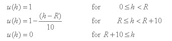
Locational variability losses The location variability is modeled by a lognormal distribution with standard deviation σL. Different values of σL are given in [1] for different environments and applications. When the receiver/mobile is located on land and outdoors but its height above ground is greater than or equal to the representative clutter height, it is reasonable to expect that the location variability will decrease monotonically with increasing height until, at some point, it vanishes. In this Recommendation, the location variability height variation, u(h), is given by:
where R (m) is the height of representative clutter at the receiver/mobile location. Therefore, for a receiver/mobile located outdoors, when computing values of the basic transmission loss for values of pL% different from 50%, the standard deviation of location variability, σL, should be multiplied by the height variation function, u(h), given in equation (11).
Building entry losses Building entry losses are defined as the difference (dB) between the mean field strength (respect to locations) outside a building at a given height above ground level and the mean field strength inside the same building (respect to locations) at the same height above ground level. For indoor reception two important parameters must also be taken into account. The first one is the building entry loss and the second one is the building entry loss variation due to different building materials. The standard deviations, given below, take into account the large spread of building entry losses but do not include the location variability within different buildings. It should be noted that there are limited reliable information and measurement results about building entry loss. Provisionally, building entry loss values that may be used are given in Table 1.
Table 1: Building entry losses, Lbe , σbe For frequencies below 0,2 GHz, Lbe = 9 dB, σbe = 3 dB; for frequencies above 1,5 GHz, Lbe = 11 dB, σbe = 6 dB. Between 0,2 GHz and 0,6 GHz (and between 0,6 GHz and 1,5 GHz), appropriate values for Lbe and σbe can be obtained by linear interpolation between the values for Lbe and σbe given in the table for 0,2 GHz and 0,6 GHz (0,6 GHz and 1,5 GHz). The field-strength variation for indoor reception is the combined result of outdoor variation (σL) and the variation due to building attenuation (σbe). These variations are likely to be uncorrelated. The standard deviation for indoor reception (σi) can therefore be calculated by taking the square root of the sum of the squares of the individual standard deviations:
where σL is the standard deviation of location variability.
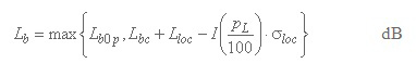
Basic transmission loss not exceeded for p% time in pL% locations The basic transmission loss not exceeded for p% time in pL% locations, Lb(dB), are:
where: Lb0p: basic transmission loss not exceeded for p% time and 50% locations associated with line-of-sight with short term enhancements . Lbc: basic transmission loss not exceeded for p% of time and 50% locations, including the effects of terminal clutter losses . Lloc: location loss median value, which is 0 dB for outdoors and equal to Lbe for indoors. I(x): inverse complementary cumulative normal distribution as a function of probability, x σloc: combined standard deviation (i.e. building entry loss and location variability), equal to σL for outdoors and given by equation (12) for indoors. REFERENCES [1] ITU-R Recommendation P.1812-1, "A path-specific propagation prediction method for point-to-area terrestrial services in the VHF and UHF bands", ITU, Geneva, Switzerland, 2009. |