DESCRIPTION

The ITU-R Recommendation P.526, “Propagation by diffraction” [1] provides several models to evaluate the effect of diffraction on the received field strength. The models are applicable to different obstacle types and to various path geometries.

DEVELOPMENT

Types of Terrain

Depending on the size of terrain irregularities, three types of terrain can be distinguished:

a) Smooth terrain: The surface of the Earth can be considered smooth if terrain irregularities are of the order or less than 0.1R, where R is the maximum value of the first Fresnel zone radius in the propagation path. In this case, the prediction model is based on the diffraction over spherical Earth (section 3).

b) Isolated obstacles: The terrain profile of the propagation path consists of one or more isolated obstacles. In this case, depending on the number of obstacles encountered in the propagation path and the idealization used to characterize them, the prediction models described in sections 4-7 should be used.

c) Rolling terrain: The profile consists of several small hills, none of which form a dominant obstruction. Within its frequency range ITU R Rec. 1546 is suitable for predicting field strength but it is not a diffraction method.

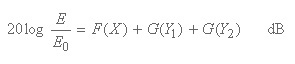
Diffraction over a spherical Earth

The calculation depends on the type of path, its distance, the frequency and the electrical characteristics of the surface of the Earth.

At long distances over the horizon, the diffraction field strength, E, relative to the free-space field strength, E0, is given by the formula:

where X is the normalized length of the path between the antennas at normalized heights Y1 and Y2 (and where 20 log E/E0 is generally negative).

For these paths, the normalized value K of surface admittance is of relevance. The appropriate formulas can be found in [1]. A graphical representation is given in fig. 1.

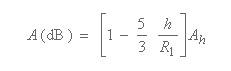
Fig. 1. Normalized factor for surface admittance K.

The detailed calculations for X, Y, F and G can be found in [1]. They are not reproduced here because of their complexity and the wide availability of ITU-R Recommendations.

In the case of LoS paths with sub-path diffraction over spherical Earth, a linear interpolation between the limit of diffraction zone (clearance of 0.6 of the first Fresnel zone radius), where the attenuation relative to free-space is zero, and the radio horizon can be used. According to this procedure, the diffraction loss is computed in terms of the first Fresnel zone radius, R1, as:

where:

h: path clearance in the range 0 to 0,6 R1

Ah: diffraction loss at the radio horizon

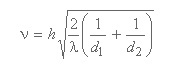
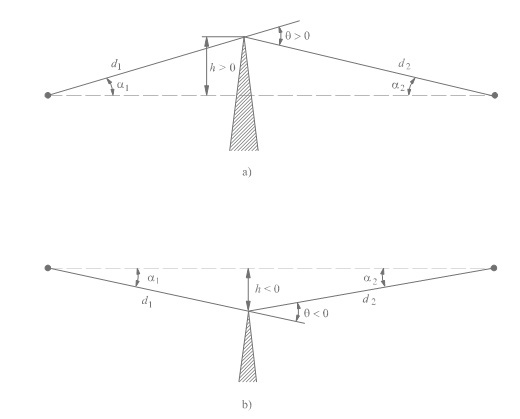
Single knife-edge obstacle

In this extremely idealized case (Fig. 2), all the geometrical parameters are combined together in a single dimensionless parameter, normally denoted by v which may assume a variety of equivalent forms according to the geometrical parameters selected. For example:

where:

h: top height of the obstacle above the straight line joining the two ends of the path. If the height is below this line, h is negative. ν has the same sign as h.

d1 and d2: distances from the two path ends to the top of the obstacle.

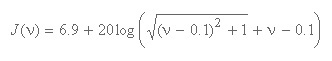
Fig. 2 Ilustration of an idealized knife-edge obstacle.

It can be shown that where R1 is the radius of the first Fresnel zone.The additional loss caused by the presence of the obstacle, J(v), depends only on v. For most practical cases (v > -0.78) it can be calculated as:

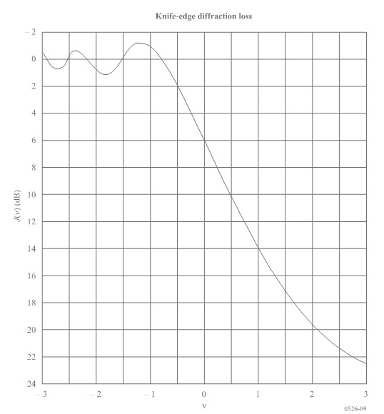
A graphical representation of J(v) is plotted in fig. 3.

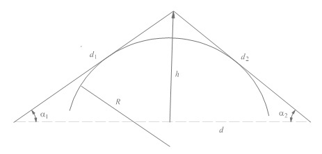
Fig. 3. Graphical representation of knife-edge diffraction loss.

Single rounded obstacle

The geometry of a rounded obstacle of radius R is illustrated in Fig. 4. Note that the distances d1 and d2, and the height h above the baseline, are all measured to the vertex where the projected rays intersect above the obstacle. The diffraction loss for this geometry may be calculated as:

where J(ν) is the Fresnel-Kirchoff loss due to an equivalent knife-edge placed with its peak at the vertex point and T(m,n) is the additional attenuation due to the curvature of the obstacle. The complete calculations can be found in the Recommendation [1].

Fig. 4. Geometrical representation of a rounded obstacle.

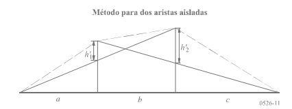
Two isolated knife-edge obstacles

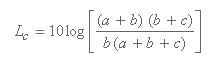
Un primer método consiste en aplicar sucesivamente la teoría de la difracción en arista de filo de cuchilloA first method consists of applying single knife-edge diffraction theory successively to the two obstacles, with the top of the first obstacle acting as a source for diffraction over the second obstacle (see Fig. 5). The first diffraction path, defined by the distances a and b and the height h'1 gives a loss L1 (dB); The second diffraction path, defined by the distances b and c and the heigh h'2 gives a loss L2 (dB). L1 and L2 re calculated using formulae of section 4.1. A correction term Lc(dB) must be added to take into account the separation b between the edges. Lc may be estimated by the following formula:

which is valid when each of L1 and L2 exceeds about 15 dB. The total diffraction loss is then given by:

The above method is particularly useful when the two edges give similar losses.

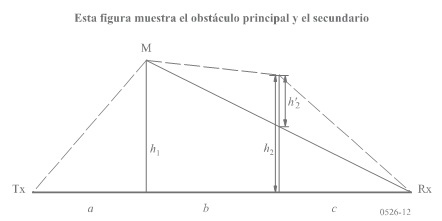
Fig. 5. Double isolated edges with similar losses

If one edge is predominant (see Fig. 6), the first diffraction path is defined by the distances a and b + c and the heigh h1. The second diffraction path is defined by the distances b and c and the height h'2.

Fig. 6. Double isolated edges with a predominant obstacle

The method consists in applying single knife-edge diffraction theory successively to the two obstacles. First, the higher h/R1 ratio determines the main obstacle, M, where h is the edge height from the direct path TxRx as shown in Fig. 6, and R1is the first Fresnel ellipsoid radius given by equation. Then h'2, the height of the secondary obstacle from the sub-path MR, is used to calculate the loss caused by this secondary obstacle. A correction term, Tc (dB), must be subtracted, in order to take into account the separation between the two edges as well as their height [1]:

The same method may be applied to the case of rounded obstacles using the corresponding calculations.

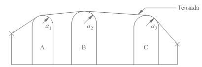
Cascaded cylinder method

In order to calculate the diffraction over multiple obstacles, this first method assumes that each obstacle can be represented by a cylinder with a radius equal to the radius of curvature at the obstacle top. This method is advisable when detailed data of the vertical profile along the ridge are available. A graphical representation is given in Fig. 7.

Fig. 7. Illustration of the cascaded cylinder method.

Having modeled the profile in this way, the diffraction loss for the path is computed as the sum of three terms:

•the sum of diffraction losses over the cylinders;

•the sum of sub-path diffraction between cylinders (and between cylinders and adjacent terminals);

•a correction term.

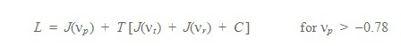
Cascaded knife edge method

This method is based on the Deygout method limited to a maximum of 3 edges. The path main obstacle p defines the division in two subpaths, with dominant obstacles t and r. The excess diffraction loss for the path is given by:

where:

J(Vp): knife-edge diffraction loss in the dominant obstacle p

J(Vp), J (Vr): knife-edge diffraction losses in the dominant obstacles t and r

C: empirical correction

C = 10.0 + 0.04 D

D: total path length (km)

and

T = 1.0 – exp [– J (Vp) / 6.0 ]

REFERENCES

[1] ITU-R Recommendation P.526-10, "Propagation by diffraction", ITU, Geneva, Switzerland, 2007.