The principle behind the profile component

The profile component is divided into two parts:

•The first one is dedicated to environments for which the polygons' geographical data is not available throughout the whole calculation zone or for occasions where you do not want to work with them.

•The second one combines the polygons' geographic data (when available) and the raster geographic data representing the surface with raster geographic data of the relief.

The calculation of the loss of propagation is almost entirely determined by the relief analysis in the vertical plane passing through the transmitter and the receiver. This hypothesis enables the transformation of each relief obstacle to a 2D theoretically thin and infinite horizontal plane and reduces it to a problem of wave diffraction calculation on a succession of thin ridges that can be treated with Fresnel formulas.

The first operation consists of elaborating the profile from the polygons' geographical data or raster geographic data representing the surface (clutter and/or clutter heights) and the raster geographic data of the relief (height).

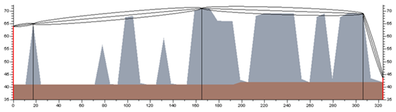
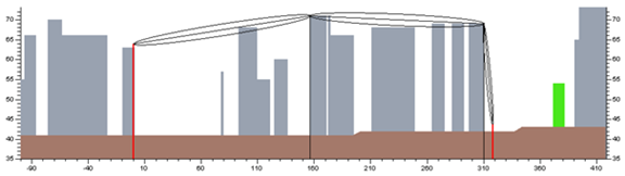
Profile example (without and with vectors)

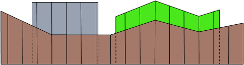
The solution chosen to construct the diffraction profile with the vectors' geographic data is to add the profile of the heights of the vectors to the altitude profile taken from the height as follows:

•For a building contour, the diffraction profile consists of ridges of equal heights. All the height ridges supporting the buildings, modified so that the building's rooftop stays flat, are increased to the height of the building. The profile is then completed with the two ridges framing the building.

•For a vegetation contour, the diffraction profile is formed from the height ridges under the vegetation contour to which the height of the contour is added. The profile is then completed with the two frame ridges of the contour where the height portion is determined by interpolation.

Once the profile is obtained so that the diffraction loss is not over-estimated, it is best to delete certain diffraction edges; therefore each diffraction edge less than one hundred meters away from a positive or negative diffraction edge is deleted. This means that a succession of diffraction edges that are so close to each other that they in fact represent only one ridge is not taken into consideration.

Deygout's method is chosen to calculate the diffraction loss. The model also calculates different variables related to the profile. The loss of the profile component results in a linear combination of these variables for which the coefficients are determined by adjusting the smallest squares with the calibration tool.

Management of raster geographic data

Raster geographical data can be of 3 different types:

•Height (Digital Terrain Model): Description of altitudes above ground of the points at the center of the pixel. This is a single point and not a calculated average on the various altitudes encountered on the pixel.

•Clutter (Digital Surface Model): Statistical description of the surface or principal theme on the pixel.

•Building raster (Digital Elevation Model): Descriptions of height above the surface of the points at the center of the pixel.

The profile component adapts itself to all types of raster data. The management of raster geographic data is based on the construction of a "height" representation and a "surface" representation.

A data representation is a zone of raster data that results from the fusion of various raster files (or from the data of one file if only one file is available) and whose construction unfolds according to the following stages:

•Inventory of the files whose intersection with the calculation area is not zero.

•Creation of a result area and positioning of each pixel to "indefinite value".

•Reading every file and fusion in the result area. During the fusion, a pixel from the resulting area is only affected if its previous value was "indefinite value".

The "height" representation is a 2D matrix that contains the description of the relief while the "surface" representation is a 2D matrix that contains the surface height (for clutter data, each type is associated with a height by the user).

The resolution of the "height" representation can be inferior, equal, or superior to that of the "clutter" representation.

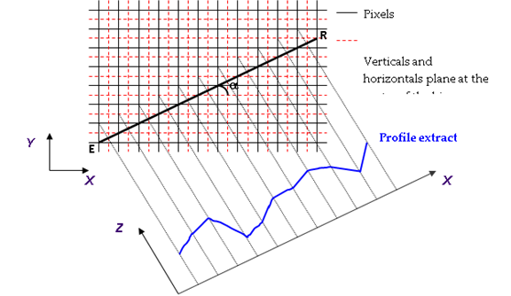
Profile extraction of raster geographical data

Taking into consideration the fact that propagation is principally done through diffraction on relief, the model constructs, in a vertical transmitter-receiver plane, a profile called "knife edge" comprised of ridges determined from the raster geographic data. For that, it extracts the profile ridges that are at the intersection points of the vertical planes (or the horizontal planes if α >=45) passing through the center of the pixels with the transmitter-receiver segment. The height of each ridge is equal to the height of the bin containing the point of intersection.

The profile is extracted by adding a value estimated by interpolating the distance starting from the surface profile to the value of each point of the height profile. At each point of the height profile, the point that provides the best frame in distance in the surface profile is chosen, and the height of the surface ridge is estimated with a linear interpolation starting from the heights and the distances from the transmitter of the "framed" ridges.

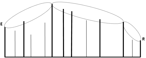
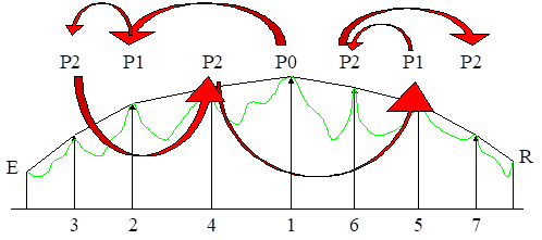
Diffraction calculation

The phenomenon of diffraction is one of the most important factors contributing to the propagation of electro-magnetic waves.

Deygout's method has been chosen for the profile component. It uses three fundamental concepts to arrive at the calculation of diffraction losses:

•The first Fresnel zone. It is generally understood that diffraction phenomena due to all obstacles situated outside this zone are negligible. The first Fresnel zone is the volume limited by the ellipsoid with starting points E and R, such as EM + MR – ER ≤ λ/2 (with M points belonging to the Fresnel ellipsoid).

•The Huygens' principle. The fundamental idea behind Deygout's method is to understand that, to go from transmitter to receiver, the wave must, by diffraction, avoid a limited number of obstacles (thin ridges) taking each one into consideration after the other in function to their importance regarding the method of the Fresnel calculation, that is to say in relation to the Fresnel zones defined in consequence.

•The superposition principle. As with other methods, the problem of diffraction on the multiple ridges is treated as a succession of diffractions on a single ridge, for which the Fresnel calculation is applicable. This approach is both empirical and intuitive.

The algorithm calculates recursively by sets of three (thus with a maximum of 15 edges of diffraction), between the transmitter and the receiver, the interference coefficient of each ridge in the Fresnel ellipsis. It conserves the ridges that have the largest interference coefficients, as well as the number of engaged ridges, and diffraction losses are calculated starting from these ridges.

The loss represented by the profile component, created by the accumulation of the different diffraction losses, is then corrected by adding the weighting of the calculated variables along the profile whose coefficients are determined by adjusting the least squares method by the calibration tool.